What Kind of Place Is Your County?
Sorted 3,128 US counties across 49 states and DC into four types of place using unsupervised K-Means clustering on 16 social vulnerability measures plus upward mobility, validated the grouping against Ward hierarchical clustering and a random forest, and then tested whether the types survive without their demographic inputs. Built with Python, scikit-learn, SciPy, pandas, Plotly, and Streamlit as a portfolio project in AI4ALL’s Ignite accelerator.
The harder question is the one the project spends most of its energy on. Are those groups real, or just an artifact of what somebody decided to measure?
I go to school at UIUC, where the gap between Downtown Champaign and Campus Town is impossible to miss. So it was a genuinely fun surprise when the model decided that Champaign County Illinois is most like Ingham County Michigan, Alachua County Florida, Tippecanoe County Indiana, Johnson County Iowa, and Charlottesville City Virginia. Every single one is a college town. They sit an average of 377 miles from Champaign, and 579 miles from each other. Nobody told this thing that universities exist. It worked that out from poverty rates, housing, and age structure alone.
Hover any county for its name and type, drag to pan, scroll to zoom. This is the real Plotly figure rather than a screenshot of one, served from this site, so it does not depend on anything staying awake. Open it full screen.
Go try it. Uncheck any measure in the sidebar and the model refits right in front of you. Turn off Minority and Limited English and watch how little actually moves.
Source code on GitHub, including the full pipeline, the tests, and the data documentation.
Contents
- What The Mobility Number Means
- Problem Statement
- How This Project Changed
- Key Results
- Methodologies
- Data Sources
- Technologies Used
- Authors
- License
- Next Steps
What The Mobility Number Means
Take every child whose parents earned at the 25th percentile nationally. Follow them to ages 31 to 37. Ask where their own household income lands as a percentile. Average that across everyone raised in a county and you get one number for the place.
It is a rank, not dollars, always between 0 and 1. A county at 0.50 raised poor kids who ended up dead average. At 0.30 they mostly stayed near the bottom.
| Value | Where | Population | |
|---|---|---|---|
| Lowest county | 0.154 | Yakutat City and Borough, Alaska | 564 |
| Champaign County IL | 0.403 | Type 2, Costly big metros | 206,525 |
| National average | 0.430 | ||
| Highest county | 0.688 | Harding County, South Dakota | 1,176 |
Look at that population column before believing the endpoints. Harding County has 1,176 people and Yakutat has 564, so the two places anchoring a 53 point scale hold about 1,700 residents between them. Every one of the top five counties is under 3,000 people and sits in North or South Dakota. All five at the bottom are in Alaska.
That is not a coincidence, it is arithmetic. A mobility estimate is an average over the children the Atlas could track, so a county with a few dozen of them produces a number that swings on almost nothing. Mobility variance falls steadily as counties get bigger: the standard deviation is 0.084 among the smallest tenth of counties and 0.041 among the largest, and the correlation between log population and distance from the national average is -0.36. Put a floor on population and the scale collapses.
| Population floor | Counties left | Highest | Lowest | Range |
|---|---|---|---|---|
| None | 3,128 | 0.688 Harding SD | 0.154 Yakutat AK | 0.534 |
| 10,000 | 2,400 | 0.614 Stark ND | 0.245 Bethel AK | 0.369 |
| 50,000 | 987 | 0.538 Stearns MN | 0.311 Richmond City VA | 0.227 |
So roughly half of that 53 point spread is small sample noise rather than real difference between places. Read the extremes as trivia and the middle as the finding.
The middle is where the argument actually lives. The middle 90% of counties are packed between 0.345 and 0.550, a band about a fifth of a point wide. That is why a 0.08 gap between two types is far bigger than it looks. It covers roughly 40% of the range almost every county actually lives in, or about 1.3 standard deviations, and it holds across thousands of counties instead of resting on one town in the Dakotas.
Champaign sits under the national average, which is a useful reminder that a county full of university is not automatically a county that lifts its own poor kids.
Problem Statement
Public health and anti poverty programs usually rank counties worst to best and send help down the list. A ranking tells you who is struggling. It has nothing to say about what kind of trouble they are in.
That difference decides whether an intervention lands. A rural county where a third of homes are mobile homes and a quarter of adults have a disability needs something completely different from a coastal metro where families are priced out of housing they could otherwise reach. Call both of them “high need” and you have thrown away the one piece of information that would tell you what to send.
The stakes here are pretty concrete. Where a child grows up measurably changes what they earn later, and county level funding decisions get made every budget cycle with a ranking as the input. If grouping counties by kind turns out to be more useful than ordering them by severity, that is a change an agency could adopt tomorrow.
There is a second problem underneath the first, and honestly it is the one this project spends most of its time on. Any grouping is a function of what you decided to measure in the first place.
The Social Vulnerability Index counts minority status as a component of vulnerability. Hand that to a clustering algorithm and it hands back a group defined by race, which a human then gives a name to. So the question worth answering was whether these groups track material conditions or ethnicity, and the project includes an experiment that could easily have been embarrassing.
How This Project Changed
It started somewhere else. The original proposal clustered counties on CDC PLACES health outcomes, which describe how sick a county is but say nothing about what happens to the children raised in it. Swapping the outcome for Opportunity Atlas upward mobility turned a description into a question, and everything downstream followed from that one change.
The bias probe was not in the original plan either. It got added once it became clear that clustering on an index which counts minority status as a component of vulnerability would hand back a group defined by race, which a human would then name. That risk is what the whole second half of this project is about.
The hardest thing that went wrong was silent. Connecticut disappeared from the dataset without an error, because the 2023 NCHS delineation replaced its eight counties with nine planning regions on new FIPS codes while the Opportunity Atlas still publishes against the old ones. An inner join losing every row of a state looks identical to a state that was never in the file. Diagnosing it meant reconciling the row count against NCHS’s own control totals, which is documented in data/README.md, and the crosswalk fix is the first item under Next Steps.
Key Results
-
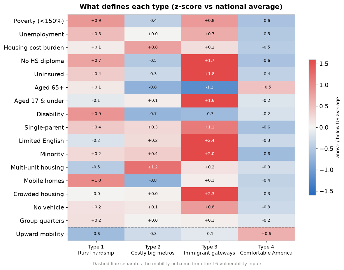
Four types of American county fell out of the data, numbered by mean upward mobility so that Type 1 is always the lowest.
Type Counties Mean mobility What stands out (z-scores) 1. Rural hardship 987 0.390 Mobile homes +1.0, disability +0.9, poverty +0.9 2. Costly big metros 630 0.412 Multi-unit housing +1.2, housing cost burden +0.8 3. Immigrant gateways 196 0.422 Limited English +2.4, crowded housing +2.3, minority +2.0 4. Comfortable America 1,315 0.470 Mobility +0.6, minority -0.6 -
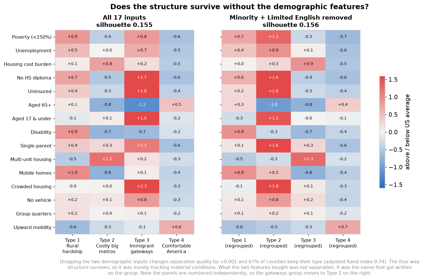
The two demographic features improved cluster separation by 0.001. Refitting without minority share and limited English moved silhouette from 0.155 to 0.156, and 67% of counties kept the type they already had (adjusted Rand index 0.735). Statistically those two columns did nothing at all. What they bought was the name that got written on the group.
-
Sixteen vulnerability measures predict 60% of the variance in upward mobility. A random forest on a held out 20% test set reached R² 0.600, MAE 0.0281, and RMSE 0.0394. That beats linear regression by ten points of R², which says the relationships are not straight lines. Unemployment on its own carries 26% of the predictive weight.
-
The 40% the model misses is where the interesting stuff lives. RMSE runs 1.40 times MAE, meaning a small number of counties get missed badly. Ranking counties by how far they beat their own prediction surfaces Stearns County MN, Ector County TX, and Starr County TX as places doing noticeably better for their poor kids than their conditions would suggest. A severity ranking buries every one of them somewhere in the middle.
-
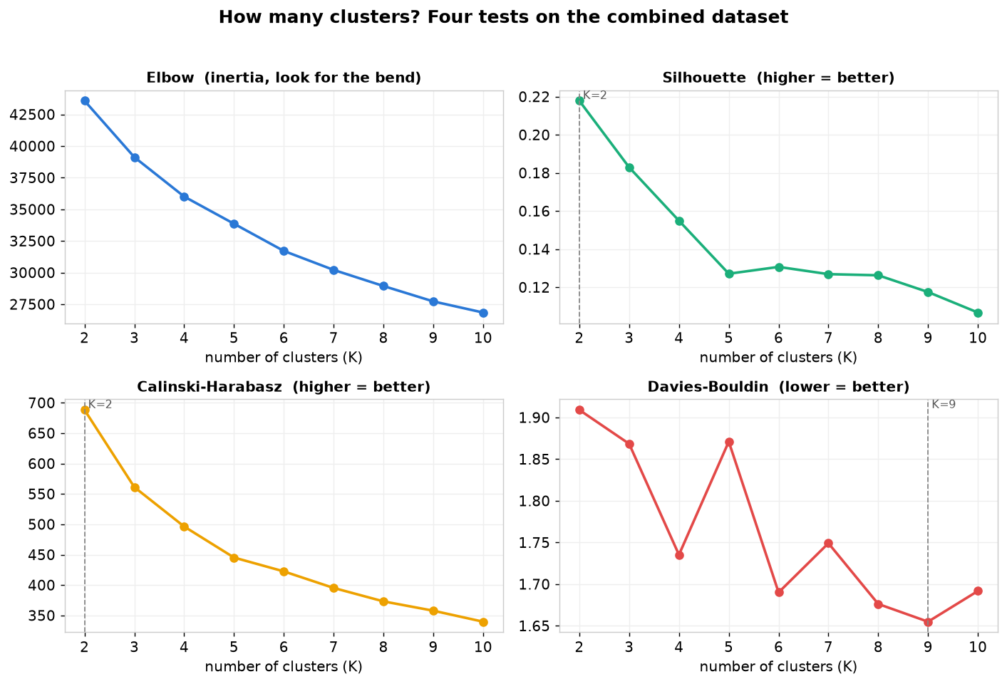
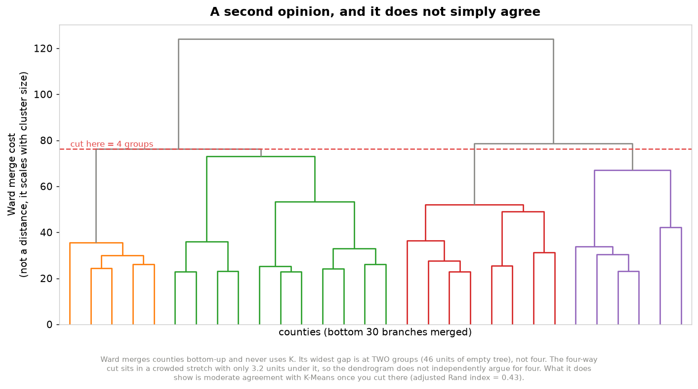
Four statistical tests for the number of clusters gave four different answers (silhouette 2, Calinski-Harabasz 2, Davies-Bouldin 9, elbow 3). The project runs 4 anyway and explains why below. Ward hierarchical clustering, which never sees K at all, does not settle it either. Its widest gap is at two groups, not four, and it only agrees with the K-Means grouping moderately once you cut it at four.
-
A live interactive version lets anybody refit the model themselves. Every checkbox drops a measure and redraws the map, so the claim that these groups depend on what got measured is something you can go test rather than something you have to take on faith.
Methodologies
Type of learning. Unsupervised clustering, with a supervised regression bolted on afterwards as a sanity check.
| Method | Inputs | Output | Why it is here |
|---|---|---|---|
| K-Means | 16 SVI measures plus mobility, standardized | one type label per county | Centroids read directly as a profile |
| PCA | the same 17 standardized features | 2 components | Only used to draw clusters in 2-D |
| Ward hierarchical | the same 17 features | dendrogram | An independent read on the structure, built without ever using K |
| Random forest | the 16 SVI measures only | predicted mobility plus importances | Do the inputs predict the outcome at all? |
Every feature gets standardized to mean 0 and standard deviation 1 before clustering. K-Means measures straight line distance, so raw percentages would let whichever column happened to have the widest range quietly run the whole show. Clusters then get renumbered by mean mobility after fitting, which keeps Type 1 as the lowest mobility group on every single run no matter what order K-Means felt like assigning its labels in.
Why K-Means, and what it costs. The centroids are the answer. Each one reads as a profile of a kind of place, and a method that produced better separated but uninterpretable groups would have been useless here.
The costs are real. K-Means assumes clusters are round and roughly the same size, which county data is not. It forces every county into some group, so there is no “this place is unlike anything else” option. K gets picked by a person rather than learned. And the whole thing sits at the mercy of feature selection and scaling, which is the weakness the bias probe goes after.
Choosing K. Follow the four tests to the letter and they send you three different directions. Silhouette and Calinski-Harabasz both point at K=2. The elbow points at K=3. Davies-Bouldin points all the way out at K=9. No value of K wins on every test, so treating this as a rule to obey does not actually settle anything.
Each test is asking its own question, which is exactly why they disagree.
| Test | What it actually measures | Wants |
|---|---|---|
| Silhouette | How much closer the average county sits to its own group than to the nearest rival group, scored from -1 to 1 | higher |
| Calinski-Harabasz | How much of the total spread in the data sits between the groups rather than inside them | higher |
| Davies-Bouldin | How badly each group overlaps with whichever neighbour it resembles most, averaged over all of them | lower |
| Elbow (inertia) | Total squared distance from every county to its own group centre, which always falls as K rises, so the signal is where it stops falling fast | the bend |
Reading all four together is a different exercise, closer to art than arithmetic.
| K | Inertia | Silhouette | Calinski-Harabasz | Davies-Bouldin |
|---|---|---|---|---|
| 2 | 43,580 | 0.2179 | 688.3 | 1.9091 |
| 3 | 39,124 | 0.1829 | 561.2 | 1.8685 |
| 4 | 36,011 | 0.1549 | 496.4 | 1.7353 |
| 5 | 33,862 | 0.1271 | 445.3 | 1.8711 |
| 6 | 31,715 | 0.1307 | 422.5 | 1.6901 |
| 7 | 30,215 | 0.1269 | 395.3 | 1.7491 |
| 8 | 28,943 | 0.1263 | 373.2 | 1.6762 |
| 9 | 27,727 | 0.1175 | 357.8 | 1.6550 |
| 10 | 26,848 | 0.1068 | 339.7 | 1.6918 |
Read the K=4 row across instead of one column at a time. Inertia is still inside its bend and K=4 is the second sharpest turn in the sweep. Silhouette and Calinski-Harabasz are both third highest of the nine. Davies-Bouldin hits a genuine local minimum, under K=3 and under K=5.
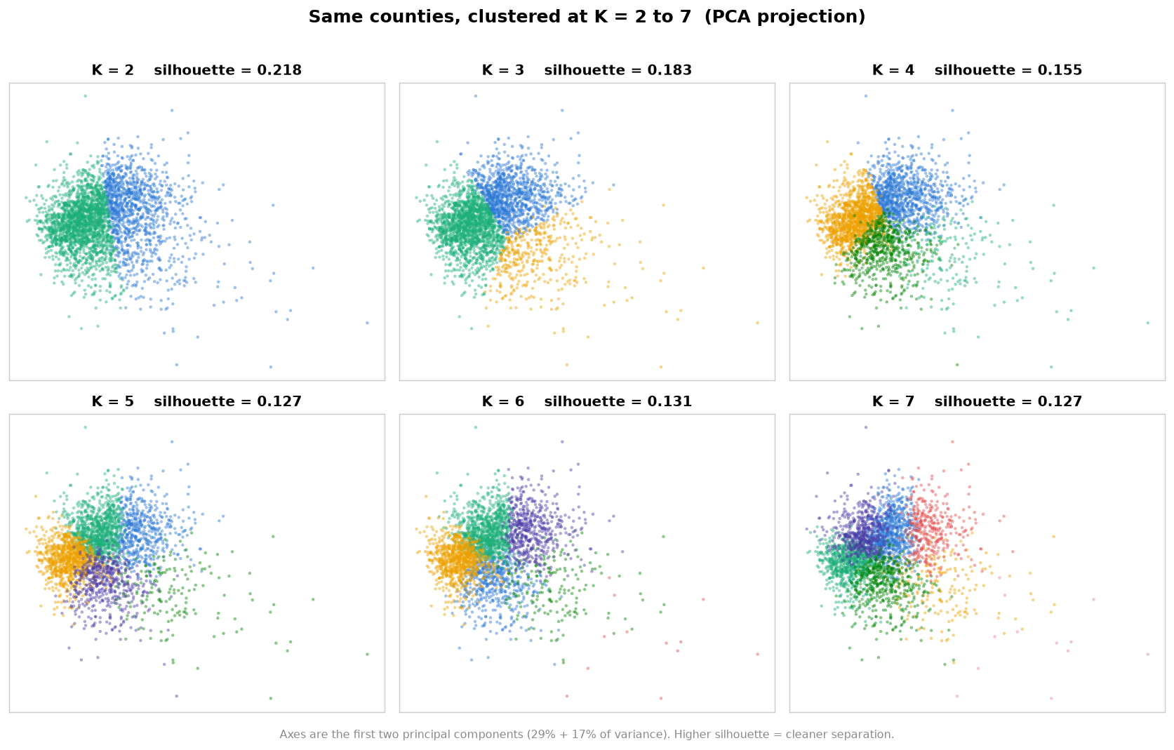
K=4 wins nothing outright. It is the only value that holds up on all four at once, which no single-test winner manages. K=2 takes the best silhouette and the worst Davies-Bouldin in the whole sweep. K=9 takes the best Davies-Bouldin and nearly the worst silhouette. On top of that, K=2 splits counties into doing fine and not doing fine, which is the same ranking this project set out to escape, and K=9 makes groups too small to fund.
Ward hierarchical clustering is a second opinion that never sees K, and it did not come back friendly. Its clearest break is at two groups, with 45.5 units of empty tree before the final merge, more than three times the runner up at six groups. The four way cut has 3.2 units under it, sixth widest of the nine, sitting in a crowded stretch where the gaps under five, four and three groups all fall within four units of each other.
Ward’s own silhouette says it louder. Cutting at two scores 0.247 and at three scores 0.224, then it drops to 0.105 at four and never climbs back. That 0.105 is worse than the 0.155 K-Means gets at the same K on the same data, so part of what Ward is saying is that its four is a bad four.
So the dendrogram does not vote for four. What it does show is moderate agreement once cut there, at an adjusted Rand index of 0.43. Immigrant gateways travels best between the two methods, though even it is not a clean match: Ward finds 177 counties where K-Means finds 196, and 127 overlap.
Ward’s real disagreement is bigger. It lumps 94% of Comfortable America together with 44% of Rural hardship into one group of 1,794. Four is a choice, not a seam the data insists on.
Evaluating the clusters. Silhouette, Calinski-Harabasz, and Davies-Bouldin all run across K=2 through 10, alongside a visual sweep of the same counties clustered at every K from 2 to 7. The sweep is the honest version of the argument. You can watch the groups hold together as K climbs and then start splitting hairs.
Each type then becomes a profile of z-scores, which is more or less the entire model in one picture.
A check the model never saw. The NCHS urban-rural code is in the dataset but is not a clustering input, so nothing about it could have influenced where the group boundaries landed. If the types are picking up something real, they should still separate on it.
| Type | Mean NCHS code | Share in a large metro (code 1 or 2) | Share metropolitan (codes 1 to 4) |
|---|---|---|---|
| 1. Rural hardship | 5.11 | 5% | 23% |
| 2. Costly big metros | 3.23 | 33% | 80% |
| 3. Immigrant gateways | 4.63 | 14% | 33% |
| 4. Comfortable America | 4.91 | 11% | 29% |
The scale runs from 1 for a large central metro to 6 for rural non core, and NCHS treats codes 1 through 4 as metropolitan. Costly big metros comes out the most urban group by a wide margin, 80% metropolitan against 23% for Rural hardship, and it is the only type where most counties sit in a metro area at all. That is outside evidence those two names describe something rather than just sounding good, and it is the only external validation in the project.
The other two types are the honest caveat. Immigrant gateways and Comfortable America land at 33% and 29%, close enough that this check says nothing useful about either.
Evaluating the supervised model. An 80/20 train test split, scored only on data the model never got to see.
| Model | R² | MAE | RMSE |
|---|---|---|---|
| Linear regression | 0.503 | 0.0323 | 0.0439 |
| Random forest | 0.600 | 0.0281 | 0.0394 |
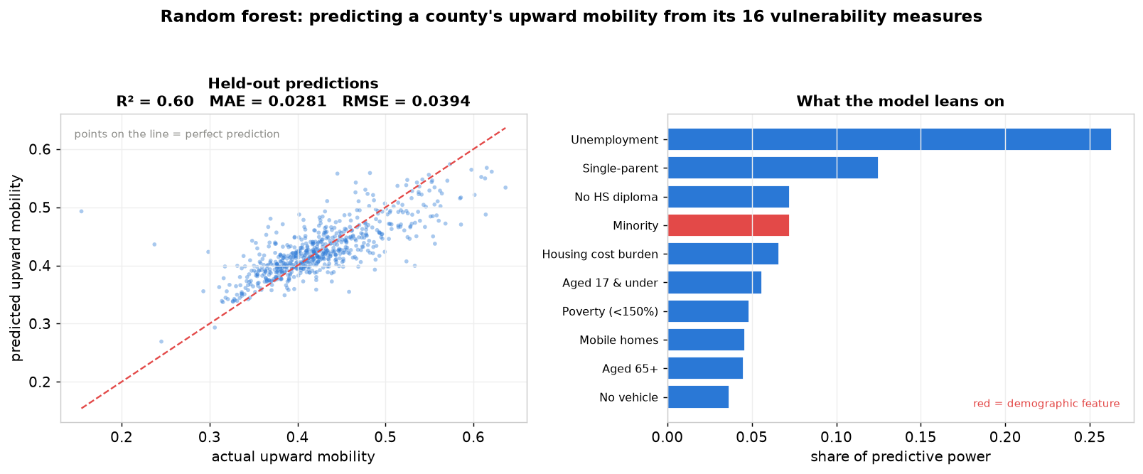
RMSE comes out 1.40 times MAE. Because RMSE squares errors before averaging, that gap says the model is not uniformly a little bit wrong. It is close on most counties and badly off on a few. Those few are exactly what the next figure is built out of.
Finding the counties that beat their odds. Predictions here come from cross validation, so no county ever gets scored by a model that trained on it, and then everything gets ranked by residual. Counties under 50,000 people are left out because their mobility estimates rest on too few children to trust.
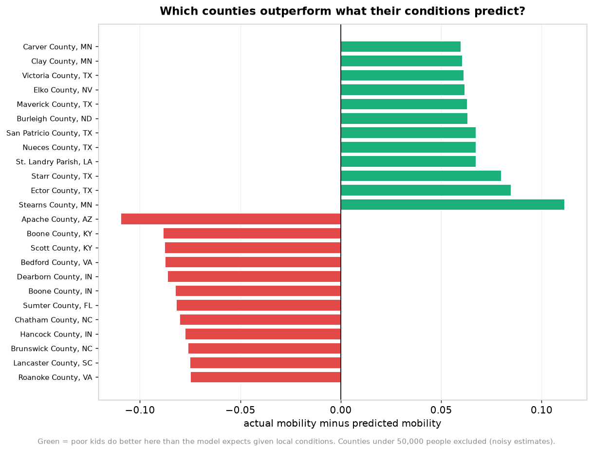
Where the two models meet. The residual is the bridge. Averaging it inside each type asks whether a whole kind of place beats or misses what its conditions predict.
| Type | Predicted | Actual | Residual | Counties above their prediction |
|---|---|---|---|---|
| 1. Rural hardship | 0.396 | 0.390 | -0.0061 | 40% |
| 2. Costly big metros | 0.415 | 0.412 | -0.0023 | 46% |
| 3. Immigrant gateways | 0.410 | 0.422 | +0.0120 | 61% |
| 4. Comfortable America | 0.464 | 0.470 | +0.0056 | 52% |
Immigrant gateways is the standout. It carries the heaviest vulnerability load of any type and its kids still beat the prediction. Rural hardship misses low. Both hold when small counties are excluded, at +0.0079 and -0.0109.
Comfortable America does not hold, and it is worth saying so. Drop everything under 50,000 people and its residual flips from +0.0056 to -0.0124, with only a third of what is left beating its prediction. The positive number in that table is coming from small counties. Whatever is going right in that type is not going right in its cities.
Tree models shrink toward the mean, which would fake exactly this by handing positive residuals to every low prediction. The correlation between prediction and residual is +0.02 and there is no drift across quintiles, so shrinkage does not explain it. Something the 16 measures miss is happening in those counties.
One caveat stands either way. Mobility is a clustering input and the forest’s target at the same time, so the types are partly defined by what the forest predicts. The forest never sees a cluster label, so the comparison holds, but the two models are not fully independent.
Testing the project’s own bias. The entire pipeline gets refit without minority share and limited English, and then the difference gets measured.
| Measure | Value |
|---|---|
| Silhouette, all 17 measures | 0.155 |
| Silhouette, minority share and limited English removed | 0.156 |
| Change in separation | +0.001 |
| Counties keeping the type they already had | 66.8% |
| Adjusted Rand index against the original labels | 0.735 |
Immigrant gateways does not disappear when the demographic columns come out. It moves. 77% of those 196 counties regroup into the second column of the right hand panel above, a group of 236 defined by crowded housing (+1.8), being uninsured (+1.8), and single parenthood (+1.6). The same places, described by what they are up against instead of by who lives there.
It shifts columns because types get renumbered by mean mobility on every fit, and the regrouped version sits at 0.400 while the costly metros group sits at 0.410. So the group that was third is now second. Worth knowing before comparing the two panels position by position, since they are sorted independently.
Run the probe yourself. The app below is the live model, not a recording. Uncheck Minority and Limited English in the sidebar and watch the silhouette delta at the top: it moves by about +0.001, and the map barely changes. That is the claim in the table above, and you do not have to take my word for it.
Hosted on Streamlit Community Cloud, which puts apps to sleep after a stretch of no traffic. If the frame above is blank or asks you to wake it, give it a minute or open it in its own tab. The figures and the map on this page are served from here and never sleep, so nothing else on the page depends on it.
How AI/ML Can Amplify or Mitigate Bias Here
There are three places bias gets into this pipeline, and the algorithm is not any of them.
What got measured. SVI counts minority status as a component of vulnerability, and CDC has defensible reasons, since these communities really do face compounded barriers during a disaster. But K-Means has no idea why a column is in front of it. Standardizing gave all 17 features equal variance, quietly announcing that a county’s minority share matters exactly as much as its unemployment rate. Nobody decided that. It was the default.
What the result got called. The model outputs the integer 2. “Immigrant gateways” came from a person. The probe shows that group is actually held together by crowded housing and lack of insurance, so a truer name is closer to “high deprivation young metros.” The first name that came to mind described who lives there rather than what they are up against, and a policymaker would walk away with a different idea about cause.
What somebody might do with it. Allocating resources by type means every county in a group gets treated identically. Aggregation bias is easy to list as a caveat. Acting on these clusters turns it into a mechanism.
Mitigation is the whole reason the probe exists. A disclaimer would have been easy and worthless, so instead there is a test whose result could have gone badly. It partly did. A third of counties change type once the demographic features come out, so they are not inert. But separation does not improve at all, so there is no performance argument for keeping them. In the live app, the checkboxes that reproduce this are the first thing anyone sees.
The case for doing this. Typing instead of ranking lets you notice that Type 3 carries high vulnerability and better than expected mobility, so copying an intervention from Type 4 into Type 1 might be exactly wrong. The residual ranking points at specific counties doing something right, and a severity ranking cannot even ask that.
The case against. Four labels over 3,128 counties is a lot of forgetting. “Comfortable America” holds 1,315 counties and plenty of them are not. A cluster label is a stereotype with a confidence interval nobody prints.
Limitations
- Mobility is historical. It tracks people aged 31 to 37 in 2014 and 2015, so they grew up in the 1980s and 1990s. The vulnerability measures and urban-rural codes are current, which means a county that was rural then and exurban now carries today’s label next to yesterday’s outcome.
- Small counties are noisy. Their estimates rest on very few children, and 23% of counties here have fewer than 10,000 people. Mobility variance runs twice as high in the smallest population decile as in the largest, which is why both ends of the national scale are tiny counties. The resilience ranking drops anything under 50,000 people. The cluster fitting does not, so every type carries some of this noise inside it.
- Correlation only. An R² of 0.60 says the features track the outcome. Nothing here shows that changing a county’s unemployment rate would change what its children earn.
- County averages hide neighborhoods. Cook County holds tracts near both ends of the national mobility range and shows up here as a single dot at 0.385, one number standing in for 5.2 million people.
- Connecticut is missing entirely. The 2023 delineation replaced its eight counties with nine planning regions on new FIPS codes, while the Opportunity Atlas still publishes against the old ones. The join found no match and the whole state fell out silently. Every national claim here is really a claim about 49 states plus DC.
- Four more counties dropped. Petroleum MT, Arthur NE, King TX and Loving TX have no mobility estimate, because they are small enough that the Atlas suppressed it. Systematic rather than random, and it points the same way as the noise problem above.
- Puerto Rico is out of scope. Its 78 municipios are in the Atlas but never entered the merge, since NCHS covers states and DC only.
- The four names are editorial. See the bias probe.
Data Sources
Three public sources joined on 5 digit county FIPS build data/county_svi_mobility.csv, 23 columns for 3,132 counties. The full data dictionary, the coverage arithmetic, and the gotchas live in data/README.md.
| Source | Contributes | What the models do with it |
|---|---|---|
| CDC/ATSDR Social Vulnerability Index | 16 EP_* measures |
Clustering inputs and the random forest’s only predictors |
RPL_THEMES, E_TOTPOP, FIPS, COUNTY, ST_ABBR |
Context, the 50,000 person filter, and the join key. None of them reach a model | |
| Opportunity Atlas | MOBILITY |
Both a clustering input and the random forest’s target |
| NCHS Urban-Rural 2023 | CODE2023 |
External validation, plus it sits in the row filter |
MOBILITY is kfr_pooled_pooled_p25 from the Atlas file county_outcomes_simple.csv, pooled across race and gender. CODE2023 runs from 1 for large central metro to 6 for non core rural, and it is the one substantive variable held out of the clustering, which is exactly why it can serve as an outside check on whether the types mean anything. SVI codes missing values as -999 rather than leaving them blank, so the pipeline nulls those before anything else runs. This extract came through clean.
References
- Chetty, R., Friedman, J. N., Hendren, N., Jones, M. R., & Porter, S. R. (2026). The Opportunity Atlas: Mapping the childhood roots of social mobility. American Economic Review, 116(1), 1-51. 10.1257/aer.20200108, also available as NBER w25147
- Flanagan, B. E., Gregory, E. W., Hallisey, E. J., Heitgerd, J. L., & Lewis, B. (2011). A social vulnerability index for disaster management. Journal of Homeland Security and Emergency Management, 8(1). 10.2202/1547-7355.1792
- Flanagan, B. E., Hallisey, E. J., Adams, E., & Lavery, A. (2018). Measuring community vulnerability to natural and anthropogenic hazards: The CDC’s Social Vulnerability Index. Journal of Environmental Health, 80(10), 34-36.
- Chetty, R., Jackson, M. O., Kuchler, T., Stroebel, J., et al. (2022). Social capital I: Measurement and associations with economic mobility. Nature, 608, 108-121. 10.1038/s41586-022-04996-4
- Chetty, R., Jackson, M. O., Kuchler, T., Stroebel, J., et al. (2022). Social capital II: Determinants of economic connectedness. Nature, 608, 122-134. 10.1038/s41586-022-04997-3
- Bowser, D. M., Mauricio, K., Ruscitti, B. A., & Crown, W. H. (2024). American clusters: Using machine learning to understand health and health care disparities in the United States. Health Affairs Scholar, 2(3), qxae017. 10.1093/haschl/qxae017
- Khan, S. S., Krefman, A. E., McCabe, M. E., Petito, L. C., Yang, X., Kershaw, K. N., Pool, L. R., & Allen, N. B. (2022). Association between county-level risk groups and COVID-19 outcomes in the United States: A socioecological study. BMC Public Health, 22, Article 81. 10.1186/s12889-021-12469-y
Technologies Used
- Python 3.14
- scikit-learn for K-Means, PCA, the random forest, the train test split, cross validated prediction, and every clustering and regression metric
- SciPy for Ward hierarchical linkage and the dendrogram
- pandas and NumPy for data preparation and the z-score profiles
- Matplotlib for seven of the eight static figures
- Plotly for the choropleth maps and every chart in the app, with Kaleido rendering the map to PNG
- Streamlit for the live explorer
Running It Yourself
python -m venv .venv
./.venv/bin/python -m pip install -r requirements.txt

./.venv/bin/python -m scripts.train       # 8 PNGs, the zoomable map as HTML, and combined_clusters.csv
./.venv/bin/python -m tests.test_app       # smoke test for clustering, type ordering, neighbours
./.venv/bin/python -m streamlit run app/app.py
scripts/train.py takes about 20 seconds, and most of that is Kaleido starting a headless browser to render the county map rather than any of the modelling. Run it before the app, because the app reads the predictions it writes out.
| Path | What it is |
|---|---|
config/config.yaml |
K, the seed, the population floor, and the feature list |
src/ |
Loading, clustering, and metrics, shared by the pipeline and the app |
scripts/train.py |
The whole pipeline, top to bottom, 8 figures |
app/app.py |
The interactive explorer |
tests/test_app.py |
Checks type ordering, ablation wiring, and the neighbour search |
data/county_svi_mobility.csv |
The merged input, 3,132 counties and 23 columns |
data/README.md |
Data dictionary and source documentation |
outputs/combined_clusters.csv |
Every county with its type, prediction, and residual |
Within a fixed environment every run of scripts/train.py produces byte identical output, so a rerun on unchanged data gives an empty diff. The one exception is figures/4_cluster_map.png. Kaleido rasterizes it through a headless Chrome that requirements.txt cannot pin, so that file moves whenever Chrome does.
Four things to do inside the app:
- Uncheck any measure in the sidebar and everything downstream refits. Dropping Minority and Limited English reproduces the bias probe live, with the silhouette delta updating as it happens.
- Run the K slider from 2 to 7, so the argument in Choosing K is something to poke at rather than take on trust.
- Click a county to pin it and light up its five closest matches, with the average distance between them.
- Rank counties against their predictions at any population floor, and diff any two counties feature by feature.
The hosted copy lives at county-cluster.streamlit.app, running on Streamlit Community Cloud against this repo’s main, so it redeploys on every push. GitHub Pages serves the write up you are reading right now, but Pages only serves static files and cannot run the app itself.
Contributing
Issues and pull requests are welcome at the repository.
- Reporting a problem. Open an issue with the command you ran and the full output. For a wrong number, say which figure or table it came from, since every claim here traces to a specific line of
scripts/train.py. - Suggesting a feature. Open an issue first. The Next Steps below are the shortlist, and the Connecticut crosswalk is the highest value one.
- Submitting code. Fork, branch, and run
./.venv/bin/python -m tests.test_appbefore opening a pull request. It checks that types stay ordered by mobility at every K, that dropping features actually changes the grouping, and that the neighbour search returns real counties. - Conventions. Four space indent, 100 character lines, double quotes, and comments that explain why rather than what. Deliberate simplifications carry a
ponytail:comment naming the ceiling and the upgrade path. - Reruns must be clean.
scripts/train.pyis deterministic within a fixed environment, sogit statusshould come back empty after a rerun on unchanged data. The one exception isdocs/figures/4_cluster_map.png, which tracks your Chrome version.
Contributions are licensed under AGPL-3.0, the same terms as the project.
Authors
Maharsh Jani (majani2@illinois.edu), University of Illinois Urbana-Champaign. Built during the AI4ALL Ignite program!
License
Copyright © 2026 Maharsh Jani. Released under the GNU Affero General Public License v3.0.
AGPL is the strongest copyleft the OSI approves, and section 13 stretches it to cover network use. Host a modified version as a web service and you owe your users the source. Since the main artifact here is a hosted app, plain GPL would have left that loophole wide open.
The underlying data is public and carries its own terms. See the Data Sources section.
Next Steps
| What | Done by | How I will know it worked |
|---|---|---|
Record the SVI extract’s release year in data/README.md, which is not written down anywhere in the repo |
Aug 20, 2026 | The vintage is stated and the ACS window is named |
| Record the demo video, 2 to 5 minutes, linked from this README | Aug 27, 2026 | Video is embedded above the fold |
| Rebuild the Connecticut join using a planning region to county FIPS crosswalk | Sep 10, 2026 | County count goes from 3,128 to roughly 3,137 and CT appears on the map |
| Weight counties by population in the resilience ranking so it stops favoring small places | Sep 24, 2026 | Comfortable America’s residual stops flipping sign when the 50,000 floor is applied |
Longer term, the residual analysis is the piece worth carrying forward. Working out which counties beat their predicted mobility is a real research question, and pairing it with the Chetty social capital measures would make it possible to test whether cross class friendship explains the gap this model leaves open.